
Section 3.1
Trapline Results
Descriptive results at the trapline level.
Landcover & Human Footprint Percentages for Traplines
The three traplines used in this project had varying amounts of human footprint, ranging from 0.2% to 10.4%. The largest contributor was Energy footprint in Trapline 1, Forestry footprint in Trapline 2, and Urban, Rural, & Industrial footprint on Trapline 3:
Trapline 1 – Energy features make up the majority of human footprint on Trapline 1, with Conventional Seismic being the top contributing feature at 0.17% of the human footprint in the area.
Trapline 2 – Forest harvest areas make up the majority of human footprint on Trapline 2, and Energy features are the next largest footprint. Among Energy features, Conventional Seismic and Pipeline (0.25%) features are the top contributors (0.71%).
Trapline 3 – Urban, Rural, & Industrial features, followed by Transportation features, make up the majority of human footprint on Trapline 3. Within the former, Clearings (of unknown purposes) occupy the largest area (1.46%). Within Transportation features, Divided Paved Roads occupy the largest area (0.52%).
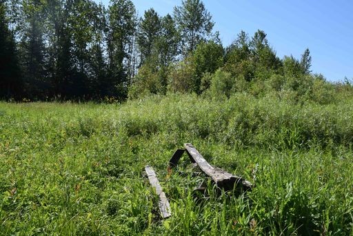
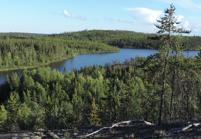
All three traplines were made up of primarily forested vegetation types:
-
Black Spruce was the most abundant habitat on all three traplines.
-
All traplines additionally had significant tracts of Deciduous Forest and Treed Fen.
-
Trapline 1 was unique in having a fairly large portion of Pine Forest (14.7%).
-
Trapline 3 had the most Black Spruce (almost 50% of its area) and a large portion of Swamp (11%).
Land Cover within each Trapline used in this Project
| Type of Cover | Area of Trapline 1 (%) | Area of Trapline 2 (%) | Area of Trapline 3 (%) |
| Vegetation | 97.9 | 93.6 | 89 |
| Bare | 0.3 | 0.0 | 0.0 |
| Water | 1.6 | 0.9 | 0.6 |
| Human Footprint | 0.2 | 5.5 | 10.4 |
| Type of Cover | Area of Trapline 1 (%) | Area of Trapline 2 (%) | Area of Trapline 3 (%) |
| White Spruce | 4.4 | 2.4 | 1.9 |
| Black Spruce | 24.0 | 28.5 | 48.6 |
| Pine | 14.7 | 5.5 | 0 |
| Deciduous | 22.9 | 17.6 | 13.6 |
| Mixedwood | 3.2 | 2.4 | 1.6 |
| Shrub | 1.4 | 0.4 | 0.0 |
| Grass | 0.1 | 0.5 | 0.1 |
| Treed Fen | 18.8 | 26.4 | 11.2 |
| Swamp | 7.2 | 5.1 | 11 |
| Open Wetland | 1.4 | 4.6 | 1.1 |
| Type of Cover | Trapline 1 (%) | Trapline 2 (%) | Trapline 3 (%) |
|---|---|---|---|
| Cumulative Burned Area 1935-2020 | 65.5 | 75.7 | 81.6 |
| Type of Cover | Trapline 1 (%) | Trapline 2 (%) | Trapline 3 (%) |
|---|---|---|---|
| Total Human Footprint | 0.2 | 5.5 | 10.4 |
| Agriculture | 0.0 | 0.0 | 0.0 |
| Energy | 0.2 | 1.3 | 1.9 |
| Forestry | 0.0 | 3.8 | 1.6 |
| Human-related Water Bodies | 0.0 | 0.0 | 0.8 |
| Transportation | 0.0 | 0.3 | 2.9 |
| Urban, Rural, Industrial | 0.0 | 0.1 | 3.2 |
Wildfire
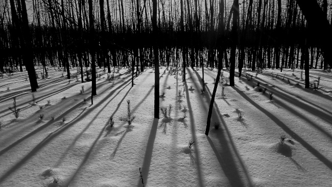
Wildfire can greatly affect the types of animals found in a given habitat, as it changes the vegetation and resources available. Some species of animals are generalists and can use burned habitats as much as non-burned ones, so are not as affected by fire. However, other species are specialists and may either show a pattern of decline in burned areas (old-growth specialists for example), or increase (disturbed area specialists).
The three traplines have all been affected by fire throughout the last century (data begin in 1935). Notably, Trapline 1 was most affected by a fire that occurred in 1981 (52.2% of its area was burned), Trapline 2 by a fire in 2016 (43.6%), and Trapline 3 by a fire in 2016 (81.6%).
| Trapline | Year | Burned Area (%) |
|---|---|---|
| 1 | 1959 | 0.8 |
| 1961 | 4.9 | |
| 1981 | 52.2 | |
| 2011 | 7.6 | |
| 2017 | 0.0 | |
| 2 | 1941 | 23.1 |
| 1943 | 0.2 | |
| 1961 | 0.5 | |
| 1998 | 8.3 | |
| 2013 | 0.0 | |
| 2016 | 43.6 | |
| 3 | 2008 | 0.0 |
| 2016 | 81.6 |
Species on the Traplines
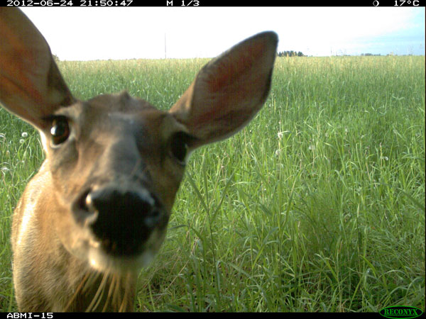
The results listed in this report are a result of 57 cameras and 22,325 images spread among the three traplines. Trapline 1 had the highest number of species (15) and Trapline 3 had the lowest (9).
Overall, Large Mammals triggered the largest number of images, with White-tailed Deer being the most common capture (11,080), followed by Moose (4,032), Black Bear (3,530), and Bison (2,187).
Furbearers triggered the next largest number of images, specifically Beaver (230) and Canada Lynx (161). A furbearer, the Wolverine, was the most rare animal captured by the cameras (1 image).
Small Mammals were also captured to some extent, though the cameras were not at an optimal height to be triggered by small-bodied creatures. Nevertheless, 140 images of Snowshoe Hare and 47 images of Red Squirrel were captured.
Finally, there were two major surprises captured by the cameras that were not expected to appear by the trappers: Striped Skunk and Raccoon.
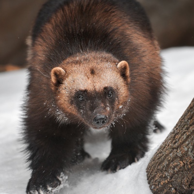
Wolverine was the most rare animal captured by the cameras (1 image).
| Trapline | Number of Cameras | Number of Images | Number of Species |
|---|---|---|---|
| 1 | 14 | 6512 | 15 |
| 2 | 25 | 9581 | 11 |
| 3 | 18 | 6232 | 9 |
Large Mammals
| Species | Number of Images |
|---|---|
| White-tailed Deer | 11080 |
| Moose | 4032 |
| Black Bear | 3530 |
| Bison | 2187 |
| Gray Wolf | 665 |
| Coyote | 122 |
Furbearers
| Species | Number of Images |
|---|---|
| Beaver | 230 |
| Canada Lynx | 161 |
| Red Fox | 83 |
| Fisher | 19 |
| Marten | 7 |
| Wolverine | 1 |
Small Mammals
| Species | Number of Images |
|---|---|
| Snowshoe Hare | 140 |
| Red Squirrel | 47 |
| Hoary Marmot | 7 |
| Weasels and Ermine | 6 |
| Voles, Mice and Allies | 2 |
Surprises
| Species | Number of Images |
|---|---|
| Striped Skunk | 4 |
| Raccoon | 2 |
Abundance of Species
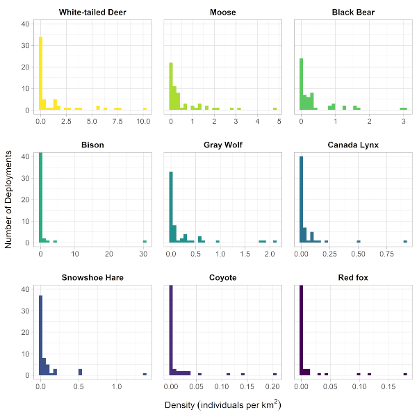
We can use cameras to estimate the abundance of various species in a given area (which we refer to as density). The important components of this calculation are the length of time the camera is operating, the total duration (time) over which each species is present in the camera field of view, and the size of area that is sampled by each camera.
This figure shows the density estimates at individual camera deployments. On the y-axis (vertical axis) of each graph, you'll see the number of cameras. On the x-axis (horizontal axis), you'll see the estimated density of each species for which data were collected. The pattern, repeated for each species, shows that low densities are associated with the majority of cameras, because most cameras are triggered infrequently by an animal passing by (it's one camera in a big area). Occasionally we see a high density for a given species at an individual camera deployment that has been triggered a lot e.g. Canada Lynx.
Over half of the deployments did not detect Canada Lynx, and the density was less than 0.1 individuals per km2 in many other deployments (which translates to a handful of images over the course of the deployment duration). However, one deployment detected lynx nine times, yielding nearly 50 photos, which resulted in an estimated density of 0.8 individuals per km2.
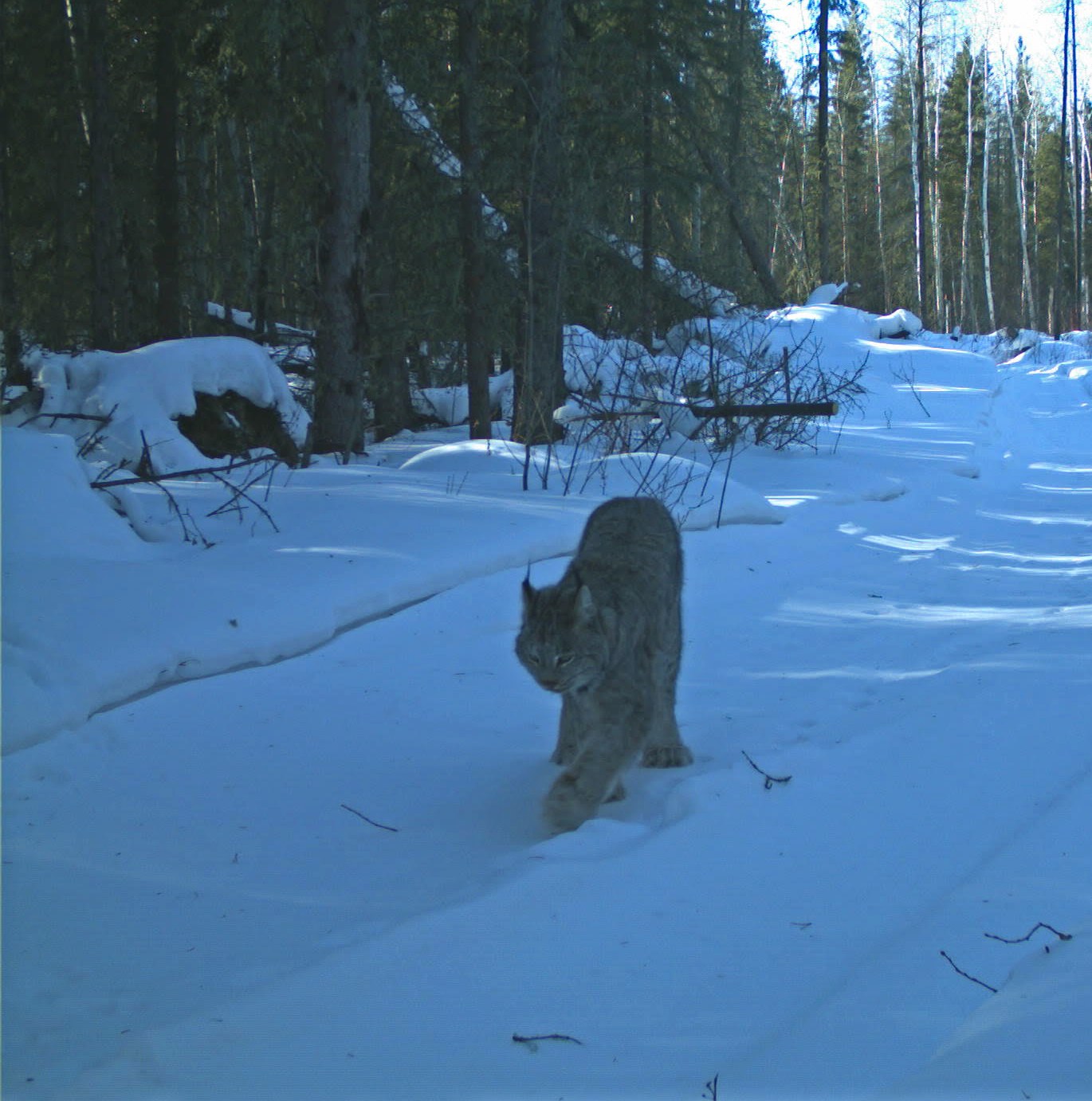
Canada Lynx had an estimated density of 0.8 individuals per km2.
Densities of Animals on Traplines
We can also calculate animal densities on each trapline. We use a simulation technique to estimate the uncertainty associated with the density estimates, reflected by the error bars around each point. In this context, ‘uncertainty’ reflects our confidence (or lack of) in each estimate. The wider the bar around a point, the less certain an estimate is. Each point can be interpreted as an estimated density for that species within that trapline, with 90% confidence that the true density value of the species lies somewhere within the range represented by the bar.
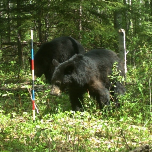
Bears were found to be most abundant on Trapline 1, and least abundant on Trapline 3.
When the error bars of two estimates do not overlap, we can be reasonably confident that the estimates are different. For example, we can see the error bars do not overlap in the density of Moose at Traplines 2 and 3; we can interpret this to mean that Trapline 3 likely has more moose. However, the estimate for Moose density on Trapline 1 is highly uncertain so we cannot be confident that Moose are more or less common on Trapline 1 than on either of the other two traplines. Conversely, it appears that Black Bears are most abundant on Trapline 1, less so on Trapline 2, and are the least abundant on Trapline 3, since the error bars do not overlap.
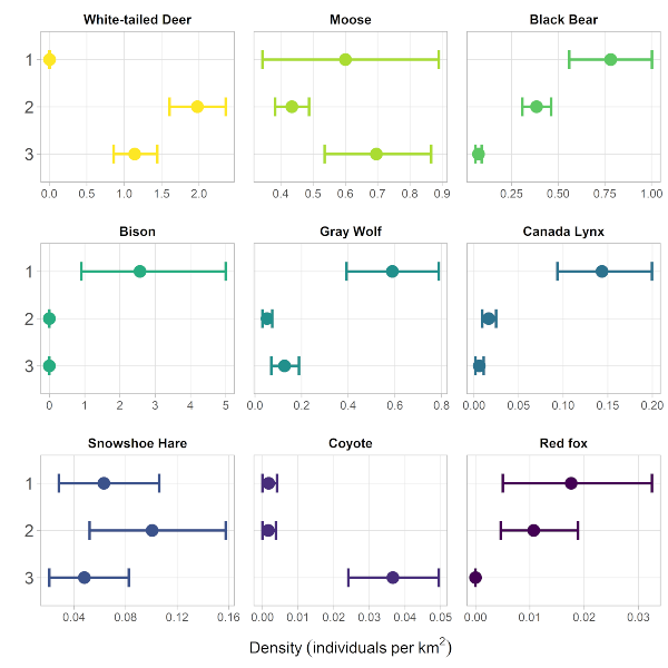
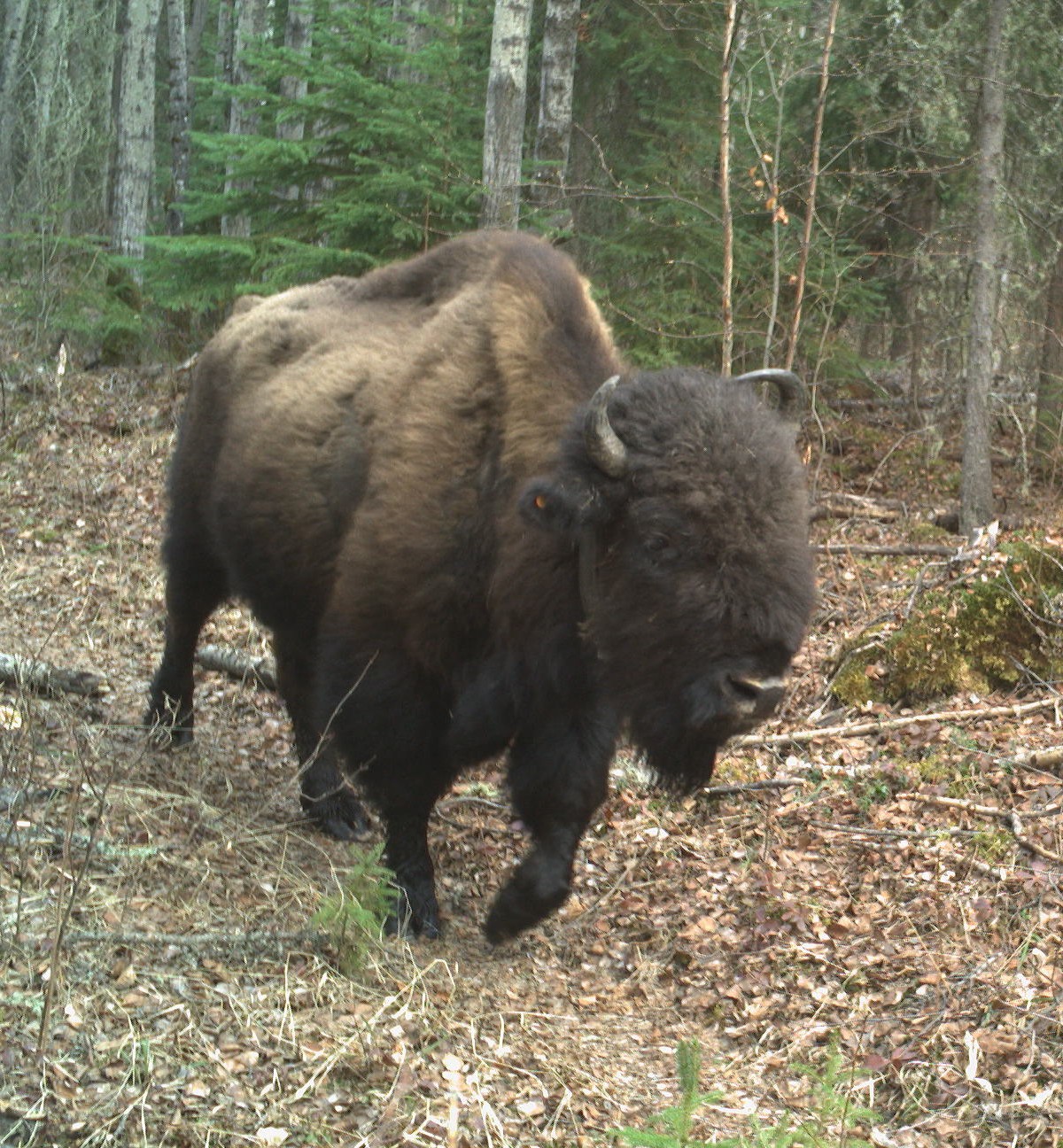
Bison were only found on one trapline.